On seeking truth and what we can learn from science

In the era where fake news is the new news, everybody seems to be constantly seeking for (their version of) “truth”, or “fact”. It is quite ironic that while we are living in a world where information is more accessible than ever, we are less “informed” than ever. However, today, let’s take a break from all the chaos in real life and see if we can learn something about “truth” from the scientific world.

3 years ago, I spent my summer interning at a laboratory on social psychology, where I was exposed, for the very first time, to statistics and the scientific methodology. That was also when my naive image of “science” shattered. It was not noble as I thought, but, as real life, messy and complicated. My colleagues showed me the dark corners of psychology research, where people are willing to do whatever it takes to have a perfect p-value and get their paper published (for example, the scandal of Harvard professor of psychology Marc Hauser). If you are somebody working in the science world, you must not be so surprised: social science, and psychology in particular, is plagued with misconduct and fraud. Reproducibility is a huge problem, as proved by the reproducibility project, where 100 psychological findings were subjected to replication attempts. The results of this project were less than a ringing endorsement of research in the field: of the expected 89 replications, only 37 were obtained and the average size of the effects fell dramatically. At the end of the internship, I wrote an article with the title “Is psychology a science ?”, where I stated in my conclusion “Pyschology remains a young field in search for a solid theoretical base, but that can not justify for the lack of rigor in the research method. Science is about truth and not about being able to publish.”

“Science is about truth”.

Is it ?

This seemingly evident statement came back to hunt me 3 years later, when I came across this quote by Neil deGrasse Tyson, a scientist that I respect a lot:

The good thing about science is that it’s true whether or not you believe in it.

That was his answer for the question “What do you think about the people who don’t believe in evolution ?”.

If we put it in the context, where he already commented on the scientific method, this phrase becomes less troubling. However, I still find it very extreme and even misleading for layman people, just like my statement 3 years ago.

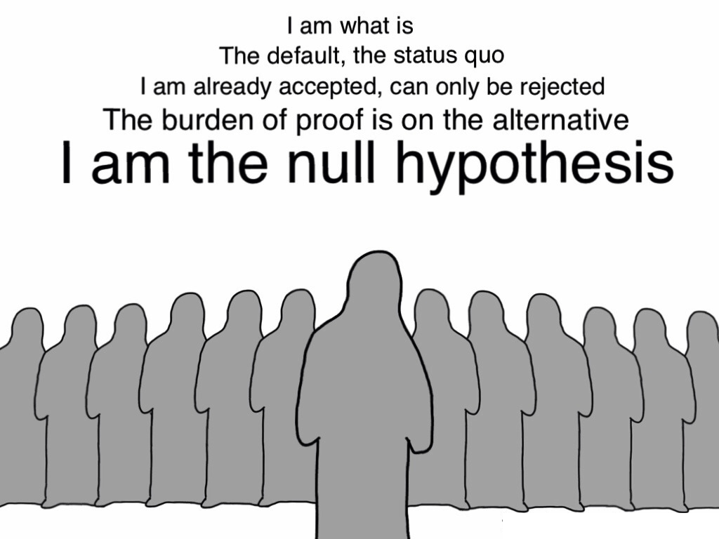
For me, science is about skepticism. It is more about not being wrong than being true. A scientific theory never aspires to be “final “, it will always be subject to additional testing.

To better understand this statement, we need to go back to the root of the scientific method: statistics.

Let’s take an example in clinical trial: supposing that you want to test a new drug. You find a group of patients, give half of them the new drug and the rest a placebo. You measure the effect in each group and compare if the difference between those 2 groups is significant or not by using a hypothesis test.

This is where the famously misunderstood p-value comes into play. It is the probability, under the assumption that there is no true effect or no difference, of collecting data that shows a difference equal to or greater than what we observed. For many people (including researchers), this definition is very counter-intuitive because it does not do what they are expecting: p-value is not a measure about the effect size, it does not tell you how right you are or how big is the difference, it just shows you a level of skepticism. A small p-value simply states that we are quite surprised with the difference between 2 groups, given that we are not expecting it. It is only a probability, so if someone try a lot of hypothesis on the data, eventually they will get something significant (this is what known as the problem of multiple comparisons, or p-hacking).

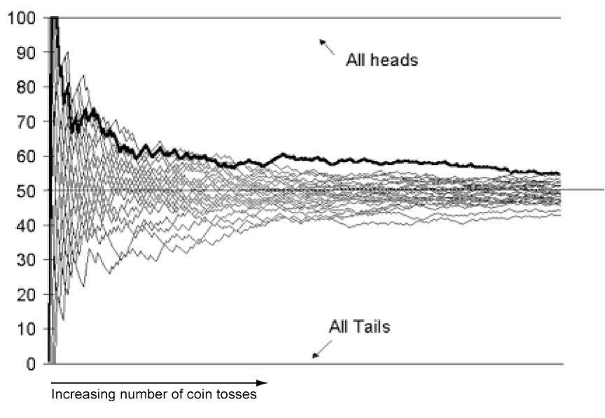
The whole world of research is driven by this metric. For many journals, a p-value less than 5% is the first criteria for a paper to be reviewed. However, things are more complicated than that. As I mentioned earlier, p-value is about statistical significance, not practical significance. If a researcher collects enough data, he will eventually be able to lower the p-value and “discover” something, even if the scope of it is extremely tiny that it doesn’t make any impact in real life. This is where we need to discuss about the effect size and more importantly, the power of a hypothesis test. The former, as it names suggests, is the size of the difference that we are measuring. The latter is the probability that a hypothesis test will yield a statistically significant outcome. It depends on the effect size and the sample size. If we have a large sample size and want to measure a reasonable effect size, the power of the test will be high and vice versa, if we don’t have enough data but aim for a small effect size, the power will be low, which is quite logical: we can’t detect a subtle difference if we don’t have enough data. We can’t just throw a coin 10 time and said that because there are 6 heads, the coin must be biased.

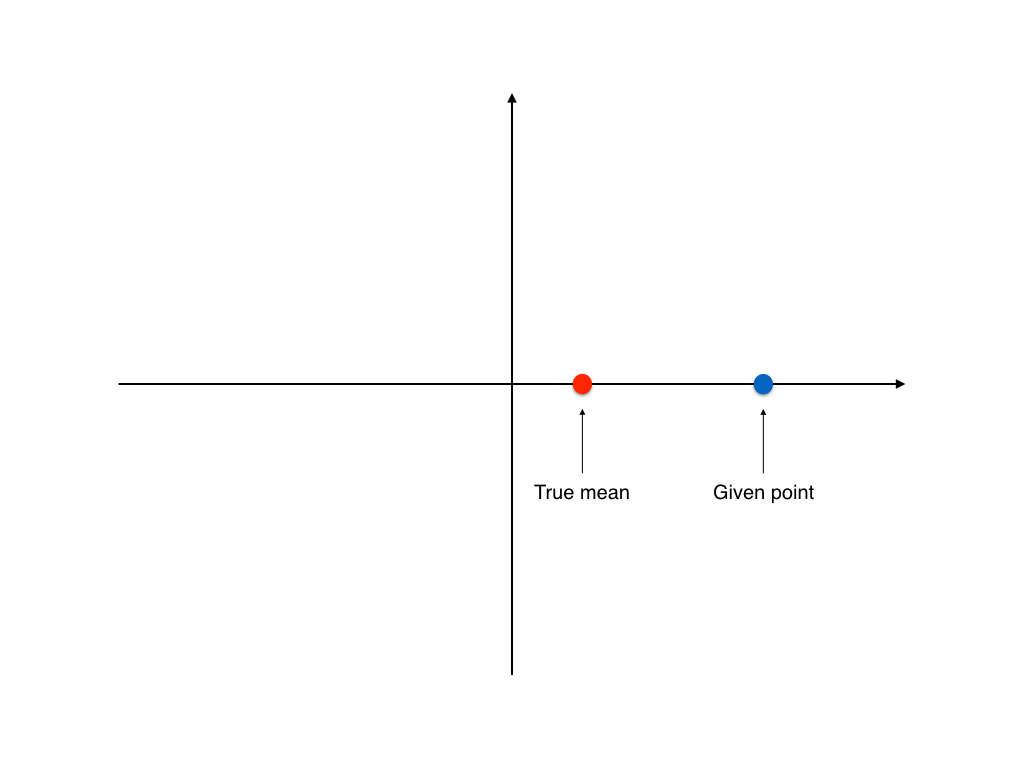
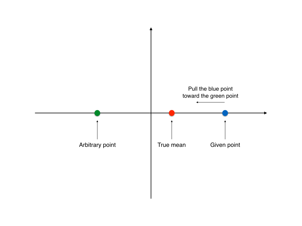
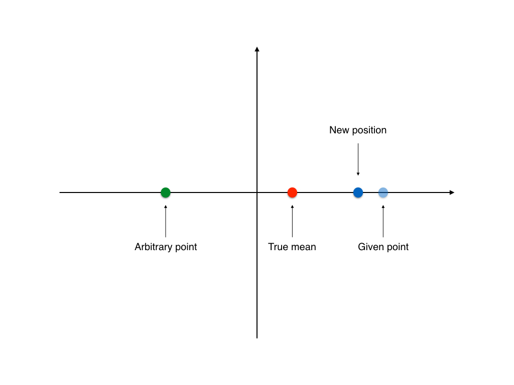
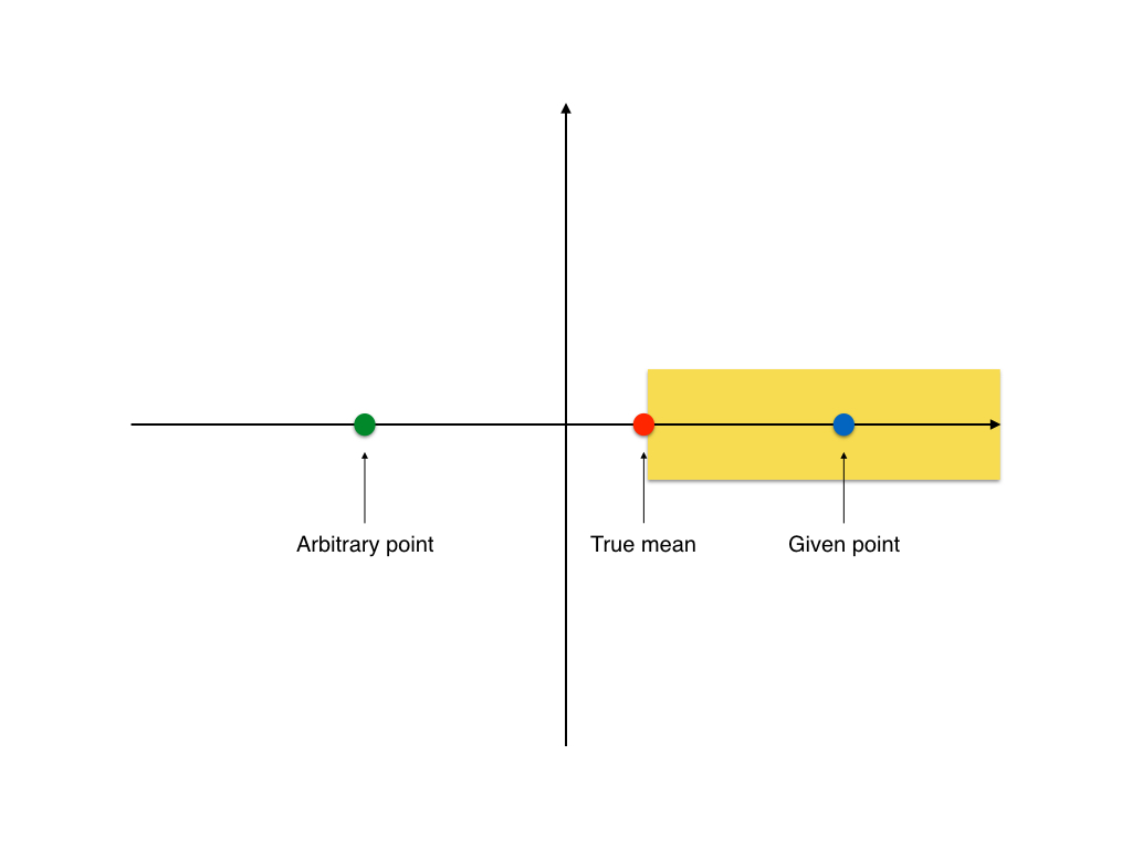
In fields where experiments are costly (social science, pharmaceutical,…), the small sample size led to a big problem of truth inflation (or type M error). This is when the hypothesis test has a weak power and thus can’t detect any reliable difference.

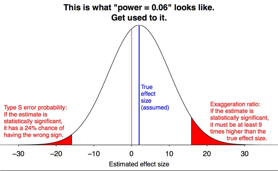
Screen-Shot-2014-11-17-at-11.19.42-AM — If we run a trial many times, we get a curve of the probability of each measured difference. The red part in the right are the required measure to have a significant result. *Source: Andrew Gelman.*

In the curve above, we see that our data needs to have an effect size 9 times greater than the actual effect size to be statistically significant.

The truth inflation problem turns out to be quite “convenient” for researchers: they get a significant result with a huge effect size! This is also what the journals are looking for: “groundbreaking” results (large effect size result in some research field with little prior research). And it is not rare.

All these discussions is to show you that scientific methodology is not definite. It is based on statistics, and statistics is all about uncertainty, and sometimes it gets very tricky to do it the right way. But it needs to be done right. Some days it is hard, some days it is nearly impossible, but that’s the way science works.

To conclude, I think that science is not solely about truth, but about evaluating observations. This is where we can go back to the real world: in this era where we are drowning in data, we also need to have a rigorous approach to process them: cross-check the information from multiple sources, be as skeptical as possible to avoid selection bias, try not to be wrong and most importantly, be honest to one self, because at the end of the day, truth is a subjective term.

On Decision and Confidence

We make many decisions every day, consciously as well as unconsciously. The term “decisions” here are not just about the high-level processes that govern how we think and asses events and observations, it is also the low-level ones that control perception and movement. For example, have you ever wondered how our body can move so smoothly ? This is definitely not an easy task if you ask any roboticists who are struggling to implement the human gaits on robots. Some scientists believe that our brain makes reliable, quick-fire predictions about the result of every movement we make, which results in a efficient sequence of actions that we call “walking”.

Confidence holds a crucial role in this process. How confident we feel about our choices will influence our behavior. If we did not have an accurate mechanism for confidence that is usually right, we would have difficulties in correcting decisions.

Important as it is, the way it works remains an unsolved riddle. The classical approach assumes that the brain takes shortcuts when processing information: it make approximations rather than uses precise statistical calculations. However, in a very recent paper, Adam Kepecs, professor of neuroscience at Cold Spring Harbor Laboratory has concluded that the subjective feeling of confidence stems from objective statistical calculations in the brain.

To determine whether the brains use objective calculations to compute the level of confidence, Kepecs created a video game to compare human and computer performance. Human volunteers would listen to streams of clicking sounds and determine which clicks were faster. Participants rated confidence in each choice on a scale of one (a random guess) to five (high confidence). What Kepecs and his colleagues found was that human responses were similar to statistical calculations. The brain produces feelings of con- fidence that inform decisions the same way statistics pulls patterns out of noisy data.

The human feeling of confience follows statistical predictions in a perceptual decision task. Source: Aam Kepecs et al.

To further examine his model, Kepecs organised another experiment in which participants answered questions comparing the populations of various countries. Unlike the perceptual test, this one had the added complexity of each participant’s individual knowledge base. Even human foibles, such as being overconfident in the face of hard choices with poor data or under-confident when facing easy choices, were consistent with Kepecs’s model.

This is not the first time a scientist suggest that our brains relies more on a statistical model than a heuristic one. In many perception tasks, it was showed that people tend to make estimates in a way that fits with Bayesian probability framework. There’s also evidence that the brain makes internal predictions and updates them in a Bayesian manner. When we read a book or listen to someone talking, for example, our brain is not simply receiving information, it is constantly analyzing this stream of data and predicting what it expects to read or hear. These predictions strongly influence what we actually read or hear. More general, we can argue that our perception of the world is in fact a reconstruction made by the brain: we don’t (or can’t ?) see the world as it is, but we see it the way our brain is expecting it.

To maintain a level of homogeneity between the real world and the “reconstructed” reality, the brain is constantly revises its predictions based on what information comes next. Making predictions and re-evaluation them seems to be a universal feature of the brain. At all times our brain is weighing its inputs and comparing them with internal predictions in order to make sense of the world.

So far we have seen some arguments support the (Bayesian) statistical paradigm. However, the scientists from the “anti-Bayesian” camp have provided a number of strong counter-arguments, especially when it comes to high-level decision making. It is fairly easy to come up with probability puzzles that should yield to Bayesian methods, but that regularly leave many people flummoxed. For instance, many people will say that if we toss a series of coins, getting all heads or all tails is less likely than getting any “seemingly random” sequence, for example, tails–tails–heads–tails–heads. It is not: as the coin tosses are independent, there is no reason to expect one sequence is more likely than another. There’s considerable evidence like the coin tosses experiment above which shows that most people are basically non-Bayesian when performing high-level, logical reasoning.

All in all, we are dealing with the most complicated thing in the known universe, and all the discovery up to know about our brain just scratch the surface. A lot of work still need to be done in order to truly understand how we think.

In conclusion, I believe that Bayesian paradigm, with its quirks and imperfections, represent a potential approach that can eventually help us see the complete picture of our brain.

Learning motor primitives on a small crawling robot using Reinforcement Learning.

Github link to the full project: Autonomous_robot_project

NB viewer link for this notebook: Learning motor primitives on a small crawling robot using Q-Learning

Binder version: Learning motor primitives on a small crawling robot using Q-Learning: go to Code\Simulation\Crawling_Simulation.ipynb

Sorry, something went wrong. Reload?

Sorry, we cannot display this file.

Sorry, this file is invalid so it cannot be displayed.

view raw QLearning.ipynb hosted with ❤ by GitHub

Gaussian Discriminant Analysis and Logistic Regression

There are many ways to classify machine learning algorithms: supervised/unsupervised, regression/classification,… . For myself, I prefer to distinguish between Discriminative model and Generative model. In this article, I will discuss the relationship between these 2 families, using Gaussian Discriminant Analysis and Logistic Regression as example.

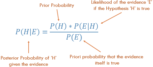
Quick review: Discriminative methods model $p(y \mid x)$ . In classification task, these models search a hyperplane (a decision boundary) seperating different classes. The majority of popular algorithms belongs to this family: logistic regression, svm, neural net, … On the other hand, Generative methods model $p(x \mid y)$ (and $p(y)$ ). This means that it will give us a probability distribution for each class in the classification problem. This give us an idea of how the data is generated. This type of model relies heavily on Bayes rule to update the prior and derive the posterior. Some well-known examples are Naive Bayes, Gaussian Discriminant Analysis, …

discriminative_vs_generative — Discriminative vs Generative. Source: evolvingai.org.

There are quite some reasons why discriminative models are more popular among machine learning practitioner: they are more flexible, more robust and less sensitive to incorrect modeling assumptions. Generative models, on the other hand, require us to define the distribution of our prior, which can be quite challenging for many situations. However, this is also their advantage: they have more “information” about the data than discriminative model, and thus can perform quite well with limited data if the assumption is correct.

In this article, I will demonstrate the point above by proving that Gaussian Discriminant Analysis (GDA) will eventually lead to Logistic Regression, and thus Logistic Regression is more “general”.

For binary classification, GDA assumes that the prior follows a Bernoulli distribution and the likelihood follows a multivariate Gaussian distribution:

$y \sim Bernoulli(\phi)$

$x \mid y=0 \sim N(\mu_0, \sum)$

$x \mid y=1 \sim N(\mu_1, \sum)$

Let’s write down their mathematical formula:

$p(y) = \phi^{y} \times (1-\phi)^{1-y}$

$p(x \mid y=0) = \frac{1}{(2\pi)^{n/2} |\sum|^{1/2} } \times exp(- \frac{(x - \mu_0)^T(x - \mu_0)}{2 \sum })$

$p(x \mid y=1) = \frac{1}{(2\pi)^{n/2} |\sum|^{1/2} } \times exp(- \frac{(x - \mu_1)^T(x - \mu_1)}{2 \sum })$

As mentioned above, the discriminative model (here is the logistic regression) try to find $p(y \mid x)$ , so what we try to prove is that:

$p(y=1 \mid x) = \frac{1}{1 + exp(-\theta^T x)}$

which is the sigmoid function of logistic regression, where $\theta$ is some function of of $\phi, \mu_0, \mu_1 and \sum$ .

Ok let’s roll up our sleeves and do some maths:

$p(y=1 \mid x)$

$=\frac{p(x \mid y=1) \times p(y=1)}{p(x)}$

$= \frac{p(x \mid y=1) \times p(y=1)}{p(x \mid y=1) \times p(y=1) +p(x \mid y=0) \times p(y=0)}$

$= \frac{1}{1 + \frac{p(x \mid y=0) \times p(y=0)}{p(x \mid y=1) \times p(y=1)}}$

This equation seems very much like what we are look for, let’s take a closer look at the fraction $\frac{p(x \mid y=0) \times p(y=0)}{p(x \mid y=1) \times p(y=1)}$ :

$\frac{p(x \mid y=0) \times p(y=0)}{p(x \mid y=1) \times p(y=1)}$

$= exp(-\frac{(x - \mu_0)^2}{2 \sum} + \frac{(x-\mu_1)^2}{2 \sum} ) \times \frac{1 - \phi}{\phi}$

$= exp(\frac{(x-\mu_1)^2 - (x-\mu_0)^2}{2 \sum}) \times exp(\log(\frac{1-\phi}{\phi}))$

$= exp(\frac{(\mu_0 - \mu_1)(2x-\mu_0-\mu_1)}{2\sum}) \times exp(\log(\frac{1-\phi}{\phi}))$

$= exp(\frac{2(\mu_0 - \mu_1)x - (\mu_0 - \mu_1)(\mu_0 + \mu_1)}{2 \sum} +\log(\frac{1-\phi}{\phi}))$

$= exp(\log(\frac{1-\phi}{\phi}) - \frac{\mu_0^2 + \mu_1^2}{2\sum} + \frac{\mu_0 - \mu_1}{\sum} \times x )$

$= exp[ (\log(\frac{1-\phi}{\phi}) - \frac{\mu_0^2 + \mu_1^2}{2\sum}) \times x_0 + \frac{\mu_0 - \mu_1}{\sum} \times x ]$

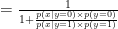
In the last equation, we add $x_0 = 1$ so that we can have the desired form $\theta^Tx$ . The former equation is then:

$\frac{1}{1 + \frac{p(x \mid y=0) \times p(y=0)}{p(x \mid y=1) \times p(y=1)}} = \frac{1}{1 +exp[ (\log(\frac{1-\phi}{\phi}) - \frac{\mu_0^2 + \mu_1^2}{2\sum}) \times x_0 + \frac{\mu_0 - \mu_1}{\sum} \times x ] }$

And there it is, we just proved that the result of a Gaussian Discriminant Analysis is indeed a Logistic Regression, our vector $\theta$ is:

$\theta = \begin{bmatrix}\log(\frac{1-\phi}{\phi}) - \frac{\mu_0^2 + \mu_1^2}{2\sum} \\ \frac{\mu_0 - \mu_1}{\sum} \end{bmatrix}$

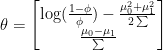
The converse, is not true though: $p(y \mid x)$ being a logistic function does not imply $p(x \mid y)$ is mutlivariate gaussian. This observation shows us that GDA has a much stronger assumption than Logistic Regression. In fact, we can go 1 step further and prove that if $p(x \mid y)$ belongs to any member of the Exponential Family (Gaussian, Poisson, …), its posterior is a logistc regression. We see now a reason why Logistic Regression is widely used: it is a very general, robust algorithm that works for many underlying assumptions. GDA (and Generative models in general), in the other hand, makes much stronger assumption, and thus is not ideal for non-Gaussian or some-crazy-undefined-distribution data .

(The problem of GDA, or generative model, can be solved with a class of Bayesian Machine Learning that uses Markov Chain Monte Carlo to sample data from their posterior distribution. This is a very exciting method that I’m really into, so I will save it for a future post.)

Human thought process from a data nerd’s point of view

This post is inspired by a late night discussion with a friend at a party (yes, because at 2am and a stomach full of mojito, there is no better topic to talk about than Machine Learning), so please take it with a grain of salt.

The ultimate goal of Artificial Intelligence is, as its name suggests, to create a system that can reason the way human does. Today, despite all the hype about Deep learning, people who work in Machine Learning and AI know that there is still a long way to go in order to achieve that dream. What we have done so far is extremely impressive, but every single modern ML algorithm is very data-intensive, which means that it needs a lot of examples to work well. Beside, in some sense, ML algorithm is just “remembering” what we show them, their abilities to extrapolate the knowledge are very limited, or nonexistent. For example, show a baby a dog, and later she can easily distinguish between a dog and a cat, even though she didn’t “know” the cat. Most of ML models can not do that, if you show them something that they have never seen, they will just try to find the most similar thing in their vocabulary to assign to it.

terminator_salvation77 — “Sorry dude, I have no idea how to create Skynet.”

Anyway, today’s topic is not about the machines. In this post, I want to take the opposite approach and compare the human thought process with a machine learning model.

For me, the way we reason and make decision follows a generative model: we compute the probability distribution for each options, and then we choose the most probable one. We use extensively Bayes’ rule to incorporate new observation into our worldview, which means that in our mind, we already have a prior probability distribution for every phenomenon. Each time we have a new information about a particular phenomenon, we will then update the corresponding prior. For example, for someone who spends his whole life in a tropical country, when he sees that it is sunny, he is 100% sure that it is hot. Now if he moves to a country in the temperate zone, he will then have to “update” his belief because in winter, it is cold with or without the sun.

bayes_theorem_1 — Bayes’ theorem. Source: gaussianwaves.com

The prior belief is what people usually call “prejudice”, and the question whether it is hard to change or not depends on each individual. I will argue that for a young, open-minded person, her “prejudice distribution” has the form of a Gaussian curve with high variance, which doesn’t have a lot of statistical strength, which allows her to update her belief easily. In contrast, someone with very low Gaussian variance has a firm belief (or prejudice), and it’s very difficult to change their mind.

normal_distribution_pdf-svg — For the same mean, a person with higher “variance” is more open-minded (the peak is lower, the tail has more weight). Source: Wikipedia.

Now let’s think about the decision making process. Just like a ML model, we use “data” to make a “prediction”. Each “data point” is a collection of many features, ie. information that can potentially affect the decision.

Before going any further, we need to talk about the “bias-variance dilemma” in Machine Learning. In his amazing article “A few useful things to know about machine learning”, Pedro Domingos gave the following explanation:

Bias is a learner’s tendency to consistently learn the same wrong thing.

Variance is the tendency to learn random things irrespective of the real signal.

note_aftml_bias_variance_in_dart_throwing — Source: “A few useful things to know about machine learning”, Pedro Domingos.

The bias-variance says that if the bias increases, the variance will eventually decrease and vice versa. This tradeoff links directly to a severe problem in ML: overfitting and underfitting.

Overfitting occurs when the model is learning from the noise and it can’t generalise well (low bias – high variance).

Underfitting is the opposite: the model is not robust enough to make any decision (high bias – low variance).

When building a model, every ML practitioner faces this challenge: find the sweet spot between bias and variance.

In my opinion, the problem with human thought process is that in auto mode, our mind is constantly “underfitting” the “data”, the reason being our mental model is too simple to deal with the complexity of life (wow I sound like a philosopher haha!). I need to emphasize the “auto mode” here because when we are conscious about the situation and focus at the task at hand, we become much more effective. However, over 90% of the decisions we make everyday is in unconscious state (just to be clear, I don’t mean that we are in a coma 90% of the time …).

The question now is: why is our mental model too simple ? From a ML point of view, I can think of 3 reasons:

Lack of data: this can seems to contradict to what I just said in the beginning about our great ability to learn well with few observations. However, I still stand my ground: humans are amazing at learning and extrapolate concrete concepts. The problem raises when it comes to the abstract, complex ones that don’t have a clear definition. In these cases, the decision boundary is a non-linear, extremely complicated one, and thus without enough data, our mind fails to fit an appropriate model.
Lack of features: this one is interesting. When building a ML system, we are usually encouraged to remove the number of features because it can help our model to generalize better and avoid overfitting. Moreover, a simpler model will need less computational power to run. I believe that our mind works in the same way: by limiting the number of features going into the mental model, it can process the information faster and more efficiently.The problem is that for complex situations, the model doesn’t have enough features to make good decisions. One obvious example is when we first meet someone. It is commonly know that we just have seven seconds to make a first impressions. Statistically speaking, this is because our mental model for first impression just takes into account the appearance as feature, it doesn’t care (at that very moment) the personality of the person, his job, or his education, …
Wrong loss function: loss function is the core element of every ML algorithm. Concretely, to improve the performance of the prediction, a ML algorithm needs to have a metric that allows it to know how well it does so far. That’s when loss function comes into play: it decides what is the “gap” between the desired output and its actual prediction. The ML algorithm then just needs to optimise that loss function.If we think about our thought process, we can see that for certain tasks, we have the wrong idea about the “loss function” since the beginning. An extreme example is when we want to please or impress someone, we begin to bend our opinions to suit theirs, and eventually our worldview is largely affected by theirs. This is because our loss function in this case is “her satisfaction” instead of “my satisfaction”. This is why people usually say that the key to success is to “fake it till you make it”: if your loss function is your success, get out of your comfort zone and do whatever the most succesful ones are doing, your mental model will eventually be changed to maximize it.

So what can we do to improve our mental model, or more concretely, to make better decisions ? This is a very hard question and I’m not at all qualified to answer it. However, for the sake of argument, let’s think about it as a ML model: what would you do if your ML model doesn’t work well ? Here are my suggestions:

Experience more: this is the obvious solution for the lack of data. By getting out of your comfort zone, stretching your mind, you will “update” your prior belief more quickly. So do whatever that challenge you, be it physically or mentally: read a book, ride a horse, run 20 km, implement a ML algorithm (my favorite ahah), just please don’t sit there and let the social media shapes your mental model.
Be mindful: as I said earlier, when we are really conscious of our actions, we can perform in a whole new level with an incredible efficiency. By being mindful, we can use more “features” than what our mental model usually takes into account, and thus we can have a better view of the situation. However, this is easier said than done, I don’t think that we can biologically maintain that state all the time.
Reflect on yourself: each week/month/year, spend some time reflecting on your “loss function”: what is your priority ? what do you want to do ? who do you want to become ? Let it be the compass for your actions, your decisions and you will soon be amazed by the results.

In conclusion, mental model is just like a ML model in production: you can not modify its output on the fly. If you want to improve its performance systematically, you need to take time to analyse and understand why it works the way it does. This is a trial-and-error, an iteration process that can be long and tedious, but it is crucial for every model.

Experience more, embrace mindfulness and reflect often, sooner or later you will possess a robust mental model. All the best!

Random thought on randomness or why people suck at long-term vision

Law of large number is one of the foundational theorem in probability theory. It says that the average of the results obtained from a large number of trials should be close to the expected value, and will tend to become closer as more trials are performed.

lawoflargenumbers — Example of Law of Large Number: tossing a coin

This theorem is very simple and intuitive. And perhaps because it is too intuitive, it becomes counter-intuitive. Why ? Let’s talk about the Gambler’s Fallacy: in a binary-result event, if there has been a long run of one outcome, an observer might reason that because the 2 outcomes are destined to come out in a given ratio in a lengthy set of trials, the outcome that has not appeared for a while is temporarily advantaged. Upon seing six straight occurences of black from spins of a roulette wheel, a gambler suffering from this illusion would confidently bet on red for the next spin.

Why is it fallacious to think that sequences will self-correct for temporary departures from the expected ratio of the respective out-comes ? Ignoring for a moment the statistically correct answer that each turn is independent from each other and imagining that the gambler’s illusion is real, we can still point out many problems with that logic. For example, how long will this effect last ? If we take the roulette ball and hide it for 10 years, when unearthed, how will it know to have a preference for red ? Obviously, the gambler’s fallacy can’t be right.

So why can’t the Law of Large Number be applied in the case of Gambler’s Fallacy ?

Short answer: Statistically speaking, humans are shortsighted creatures.

Long answer: People generally fail to appreciate that occasional long runs of one or the other outcome are a natural feature of random sequences. If you don’t buy it, let’s do a small game: take out a small piece of paper and write down a sequence of random binary number (1 or 0 for example). Once you are done, count the length of the longest run of either value. You will notice that that number is quite small. It has been demonstrated that we tend to avoid long runs. The sequences we write usually alternate back and forth too quickly between the two outcomes. This appears to be because people expect random outcomes to be representative of the process that generates them, so that if the trial-by-trial expectations for the two outcomes are 50/50, then we will try to make the series come out almost evenly divided. People generally assume too much local regularity in their concepts of chance, or in other terms, people are lousy random number generators.

So there you are, we can see that human, in nature, are statistically detail-oriented. We don’t usually consider the big picture but regconize only some “remarkable” details which will shape our point of view about the world. When we meet a new person, the observations of a few isolated behaviors leads directly to judgments of stable personal characteristics such as friendliness or introversion. Here it is likely that observations of the behavior of another person are not perceived as potentially variable samples over time, but as direct indicants of stable traits. This problem is usually described as “The Law of small number”, which refers to the tendency to impute too much stability to small-sample results.

Obviously, knowing about this won’t change our nature, but at least once we acknowledge about our bias, we can be more mindful of the situation and of our decisions.

Stein’s paradox or the power of shrinkage

Today we will talk about a very interesting paradox: the Stein’s paradox. The first time I heard about it, my mind was completely blown. So here we go:

Let’s play a small game between us: supposing that there is an arbitrary distribution that we have no information about, except that it is symmetric. Now we are given a sample of that distribution. The rule is simple, for each round, each one of us will, based on the given sample, guess what the distribution’s mean is, and whoever has the estimated point closer to the true mean get 1 point. The game has many rounds, and who wins more rounds will be the final winner.

The first time I heard about the game, I have no idea what is going on. The rule is dead simple, and it seems completely random, there is no information whatsoever to find the true mean. The only viable choice is to take the sample as our guess.

However, it turns out that there is a better strategy to win the game in a long run. And I warn you, it will sound totally ridiculous.

Ok you’re ready ? The strategy is to take an arbitrary point, yes, any point that you like, and “pull” the the sample value toward it. The new value will be our new guess.

So if you look at the image below, you can see that by pulling the given point, our new guess is closer to the mean, and thus I win!

But..but…you will tell me that had I chosen the arbitrary point on the right of the given point, I would have lost! That’s totally correct ahah!

However, let’s take a step back and look at the big picture: given the position of the arbitrary point, my strategy will beat the naive approach if the given sample is on the right of the true mean (yellow zone in the image bellow).

But that is still not enough to win the game in the long run you say ? Brace yourself, here comes the magical part: I will win too if the sample point is on the left of the arbitrary point, because in that situation, the sample will be pulled toward its right, and is thus closer to the true mean. So in long run, with my ridiculous strategy, I will win more time than you!

This paradox shows us the power of shrinkage: even if we shrink our “estimation” with an arbitrary, completely random value, we will still have a better estimation in the long run. That’s why shrinkage method is widely used in machine learning. It is just that magical!

[Fr] Système de recommandation

While cleaning my hard drive, I stumbled upon my very first Data Science project. I implemented a recommander system for a website using Collaborative Filtering. It was fascinating and frustrating at the same time as I was struggling for a several weeks, trying to wrap my head around the techniques like Stochastic Gradient Descent and Alternative Least Square. Looking back, I have come quite a long way in 1 year. However, many exciting things are still waiting for me ahead, and I can’t wait to face my next challenge!

Recommender system: article. Enjoy!

Multicollinearity in Regression Model

Multicollinearity occurs when two or more predictors in the model are correlated and provide redundant information about the response. This is a common situation in real life regression problem and depending on the goal of the user, it can be more or less troublesome.

If the goal is simply to predict Y from a set of X variables, then multicollinearity is not a problem. The predictions will still be accurate, and the overall $R^2$ (or adjusted $R^2$ ) quantifies how well the model predicts the Y values. If the goal is to understand how the various X variables impact Y, then multicollinearity is a big problem.

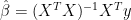
We begin with the linear regression model. The most basic one uses Ordinary Least Square technique to estimate the regression coefficients. The solution of a OLS linear regression is given by:

$\hat{\beta} = (X^TX)^{-1} X^T y$

Note here that if $X$ is not full rank (ie. the predictors are not independent from each other), $X^TX$ is not invertible, and thus there is no unique solution for $\hat{\beta}$ . This is where all the troubles begin. One problem is that the individual P-values can be misleading (a P-value can be high, even though the variable is important). The second problem is that the confidence intervals on the regression coefficients will be very wide. The confidence intervals may even include zero, which means one can’t even be confident whether an increase in the X value is associated with an increase, or a decrease, in Y. Because the confidence intervals are so wide, excluding a subject (or adding a new one) can change the coefficients dramatically and may even change their signs.

The unstable P-value can lead to some misleading and confusing results. For example, if we have 2 correlated predictors, we might stumble upon an extreme situation in which the F-test confirms that the model is useful for predicting $y$ , but the coefficient t-tests are non-significant, which suggest that none of the two predictors are significantly associated to $y$ ! The explanation is quite simple: given that $\beta_1$ and $\beta_2$ are 2 the estimated coefficients, $\beta_1$ is the expected change in y due to $x_1$ given $x_2$ is already in the model and vice versa, $\beta_2$ is the expected change in y due to $x_2$ given $x_1$ is already in the model, since both $x_1$ and $x_2$ contribute redundant information about $y$ once one of the predictors is in the model, the other one does not have much more to contribute. This is why the F−test indicates that at least one of the predictors is important yet the individual t-tests indicate that the contribution of the predictor, given that the other one has already been included, is not really important.

Statistically speaking, a high multicollinearity will inflate the standard error of estimates of the predictors (and thus decrease the reliability). Consequently, multicollinearity results in a decline in the t-statistic (because $t = \frac{\hat{\beta}}{SE(\hat{\beta})}$ ). This means that the power of the hypothesis test—the probability of correctly detecting a non-zero coefficient—is reduced by collinearity: a predictor with a small coefficient might be “masked”, even if it is statistically significant.

So we can see that the biggest problem with multicollinearity is that the predictor coefficients have a large variance, and thus it is very hard to interpret their effect.

There are many methods that have been proposed to overcome this problem. Some people suggest to drop the correlated variables. However this is a very risky method because

As the variable coefficients are not stable, we are not sure which variables are the most suitable ones to be dropped, and moreover, removing one variable will cause the other correlated variable coefficients to change in an unpredicted way.
If we use step-wise regression for variable selection, we risk to overfit the dataset. (in general, step-wise methods are not recommended.)

Another direction is to use shrinkage methods, especially ridge regression. The solution to the ridge regression problem is given by:

$\hat{\beta} = (X^TX + \lambda I)^{-1} X^T y$

At the beginning we have said that in the linear regression model, the OLS estimates do not always exist because $X^TX$ is not always invertible. With ridge regression, the problem is solve: For any design matrix X, the quantity $(X^TX + \lambda I)$ is always invertible; thus, there is always a unique solution $\hat{\beta}$ .

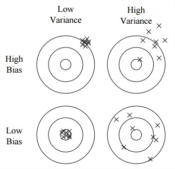
Ridge regression use the regularizer $\lambda$ to penalize large coefficients. Being a biased estimator, it trades some degree of bias to reduce the variance, and therefore results in more stable estimates.

Chi-squared distribution revisited

Today, while reviewing the regression techniques in the ESL book (Element of Statistical Learning, btw this book is pure gold, I highly recommend it!), I stumbled upon the chi-squared distribution. Concretely, the author shows that:

$(N-p-1) \hat{\sigma}^2 \sim \sigma^2 \chi^2_N-p-1$

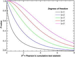
a chi-squared distribution with $N-p-1$ degrees of freedom, with $\hat{\sigma}^2$ an unbiased estimate of $\sigma^2$ .

They use these distributional properties to form tests of hypothesis and confidene interval for the parameters $\beta_j$ .

It has been a very long time since I saw the chi-squared ditribution, and of course my understanding of it becomes quite rusty. So I think this is a good chance to revisit this important distribution.

Before talking about the chi-squared distribution, we need to review some notions. First, we have the gamma function:

For $\alpha > 0$ , the gamma function $\Gamma(\alpha)$ is defined by:

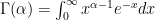
$\Gamma(\alpha) = \int_0^\infty x^{\alpha-1}e^{-x}dx$

and for any positive integer $n$ , we have: $\Gamma(n) = (n-1)!$ .

Now let:

$f(x,a) = \frac{x^{\alpha-1}e^{-x}}{\Gamma(\alpha)}$ if $x \geq 0$

and

$f(x,a) = 0$ otherwise.

Then $f(x,a) \geq 0$ . The gamma function implies that:

$\int_0^\infty f(x,a)dx = \frac{\Gamma(\alpha)}{\Gamma(\alpha)} = 1$

Thus $f(x,a)$ satisfies the 2 basic properties of a probability distribution function.

We will now use this function to define the Gamma distribution and then the Chi-squared distribution.

A continuous random variable X is said to have a Gamma distribution if the pdf of X is:

$f(x;\alpha,\beta) = \frac{1}{\beta^\alpha \Gamma(\alpha)} x^{\alpha-1} e^{-x/\beta} for x \geq 0$

and

$f(x;\alpha,\beta) = 0$ otherwise

where the parameters $\alpha$ and $\beta$ are positive. The standard Gamma distribution has $\beta = 1$ , so the pdf of a standard gamma is given by the $f(x,a)$ given above.

The Gamma distribution is widely used to model the extent of degradation such as corrosion, creep, wear or survival time.

The Gamma distribution is a family of distribution. Both the Exponential distribution and Chi-squared distribution are special case of the Gamma.

As we can see, the gamma distribution takes two arguments. The first ( $\alpha$ ) defines the shape. If shape is close to zero, the gamma is very similar to the exponential. If shape is large, then the gamma is similar to the chi-squared distribution.

Now we will define the chi-squared distribution.

Let $\nu$ be a positive integer. Then a random variable $X$ is said to have a chi-squared distribution with parameter $n$ if the pdf of $X$ is the gamma density with $\alpha = \nu /2$ and $\beta = 2$ . The pdf of a chi-squared rv is thus:

$f(x,\nu) = \frac{1}{2^{\nu/2}\Gamma(\nu/2)}x^{\nu/2}e^{-x/2} for x \geq 0$

and

$f(x,\nu) = 0$ otherwise

The parameter $\nu$ is called the degrees of freedom df of X.

The chi-squared distribution is important because it is the basis for a number of procedures in statistical inference. The central role played by the chi-squared distribution in inference springs from its relationship to normal distributions. Concretely, the chi-squared distribution is the distribution of a sum of the squares of k independent standard normal random variables. For example, in the case of linear regression, the variable $(y_i - \hat{y}_i)$ follow a normal distribution, thus to model the variance of X, which is the sum of the square of these values, we use a chi-square distribution.

The chi-squared distribution is the foundation of chi-squared tests. There are 2 types:

The goodness-of-fit test.
The test of independence.

Perhaps we will look at these tests in details in another post.